Frequently Asked Questions#
Setup & Settings#
How large should the ranges be?#
Ideally, the optimum is exactly in the center of the range and the playing strength of the engine gets worse in all directions. Obviously we do not know the optimum in advance. Thus, we usually want to err on the side of slightly too large ranges.
- Example 1#
We have one parameter and suspect it to lie in between 1 and 2, but are not 100% certain. We set the parameter range to
Real(0.0, 3.0)to avoid missing the optimum. A range ofReal(0.0, 10.0)or evenReal(0.0, 100.0)would have been overkill and likely hurt the convergence.- Example 2#
We have a parameter which lies in the range [0, 1], but are not even sure what the correct order of magnitude is (e.g. could be 0.3 or even 0.001). Here it is useful to specify a range like
Real(1e-4, 1, prior=log-uniform). Without the prior, it will be almost impossible or the tuner to find an optimum close to 0. The lower bound needs to be a value strictly larger than 0 though, otherwise applying the log-transform will result innanvalues.
Note
You can increase the ranges in your tuning configuration later in the process. You only need to restart the tuner and it will start exploring the new regions. Decreasing the ranges is possible as well, but potentially results in a loss of data (i.e. all data points outside of the new ranges are discarded).
Should I decrease the ranges late in the tune to “zoom in”?#
In general you should be very careful with zooming in to the optimum. Even though it can appear that nothing bad should happen when removing bad regions, it can actually destabilize the model for quite a few iterations. The reason is that bad regions have a lot of leverage and help inform the model about the curvature of the space and the location of the optimum.
When should you consider zooming in? If the optimum is in a very small region of the space (below 10%) and the rest of the landscape is either flat or of constant slope, it can help to zoom into the relevant region. Make sure that you do not remove the bad regions around the optimum when doing so.
Is it possible to change the acquisition function during the tune?#
Yes, this is possible without any problems and helpful in some situations. Here are a few examples:
Do you think that the overall landscape is not explored well enough? Then switch to
"vr"for a few iterations.Do you think the tuner has found the rough location of the optimum and you want to refine it? Then switch to
"mes","ei"or even"mean"for the final iterations.
How many iterations should I run? How many rounds should I run per iteration?#
The answer to this questions depends on a variety of factors: The number of parameters you want to tune, the overall effect the parameters have on the Elo performance, and how close in Elo performance you want to be to the global optimum. If you are familiar with the Stockfish Testing Queue, you already know that it takes many games to confidently decide whether a new patch improves the Elo performance of an engine. When you are tuning, you can think of this number of games as the lower bound, because now you have to basically test a large space of configurations. Due to the smoothness of this space, we can get away with fewer games, since similar configurations will likely have similar Elo performance.
A rough rule of thumb is that you should run at least 30000 * n_params games.
The volume of the search space blows up exponentially with the number of
parameters, which is why you likely need slightly more with more parameters.
You can adjust this number based on your specific parameters. If your parameters
are not very optimized, expect them to have a large impact on the Elo performance
and only want a ballpark estimate of the optimum, you can run fewer games.
If your parameters are well-optimized already, and the potential Elo gain is
in the single digits, you should run more games.
Regarding the number of rounds per iteration, consider that the computing overhead
of the tuner will ramp up with the number of rounds. A good rule of thumb is to
aim for 1000 to 1500 iterations in total. So, for example, if your goal is to
run 100k games, and want to run the tuner for 1000 iterations, then you should
set "rounds" to 100000 / 1000 / 2 = 50.
In any case, you should monitor the suite of plots and the log output, to make sure that the tuning process has converged.
How do I know if the tuning process has converged?#
There are several indicators that can be used to check whether the tuning process has converged:
Check the optima plots to see if the predicted optimal parameter values do not have a visible trend and roughly follow a tight random walk. There should also no jumps between different local optima anymore.
Check the landscape plot to see if the sampled points have formed a concentrated distribution around the optimum. The orange and red dots (corresponding to the global optimum and the conservative optimum) should be close to each other.
Check the log output to see if the confidence intervals for the parameters are not too wide.
Ensure that the confidence interval of the predicted Elo performance aligns roughly with the targeted optimality.
Can I increase the number of games per iteration later in the tune?#
It is possible, but it will bias the estimated Elo values to slightly more extreme ones. This could lead the model to temporarily over-/underevalute certain regions until enough new data points were collected.
How can I pass my own points to the tuner to evaluate?#
Note
The parameter values have to be within the bounds specified in the config file.
Starting with 0.9.2, you can pass your own points to the tuner to evaluate.
To do this, you need to create a .csv file using the --evaluate-points
option (-p for short).
Each row in the file should contain the parameters
in the same order as specified in the config file of the tune.
It is also possible to add an additional integer column to the file, which
will indicate the number of rounds to run each point for.
Here is an example of how a .csv file for a three parameter tune could look like:
0.3,125,0.0,25
0.4,1000,0.5,50
0.5,1000,0.0,50
The first point would be evaluated using 25 rounds (50 games), while the second and third point would be evaluated using 50 rounds (100 games).
Problems while tuning#
The computational overhead of the tuner has become too high? What can I do?#
There are a few things the tuner computes, that cause computational overhead. In general, the model the tuner uses (a Gaussian process) computation-wise scales cubicly with the number of iterations. Here is the list of the things which can cause a slowdown:
The estimation process of the kernel hyperparameters.
The computation of the predicted global optimum.
The computation of the optimization landscape plot.
To reduce the impact of (1.) you can reduce "gp_burnin" to a lower value
(say 1-5, even 0 late in the tuning process).
During later iterations, the model is quite sure about the kernel
hyperparameters, so it is not necessary to have a high burnin value anymore.
In the same vain, you can reduce "gp_samples" to the lowest value of 100.
Regarding (2.), you can reduce the frequency of how often the current tuning
results are reported, by setting "result_every" to a higher value or even
to 0. You can later on interrupt the tuner, and re-run it with the setting set
to 1, to force it to compute the current global optimum.
Similarly, you can reduce the frequency of the plots (3.),
by setting "plot_every" to a higher value or to 0.
A few other settings have a minor impact on the computational overhead, and could also be changed to speed up the tuning process. This will degrade the quality of the tuning process however:
Turning off
"warp_inputs"will greatly reduce the number of hyperparameters to infer, but it will also make the model less able to fit optimization landscapes with varying noise levels.Reducing the number of points
"n_points"will reduce the overhead of computing the acquisition function, but it will also make the tuning process more noisy.
Plots#
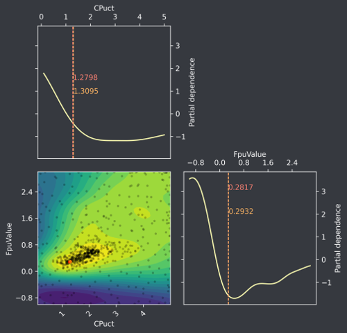
Fig. 1 Example optimization landscape for a two parameter tune.#
What is the partial dependence shown in the plots?#
First of all, the plots show the negative Elo score (the optimizer expects a function to minimize) divided by 100. Thus, lower values correspond to stronger regions of the space. Now often we want to visualize a complicated optimization landscape with more than 2 parameters. This is where we use the concept of partial dependence. A partial dependence plot shows the marginal effect a set of parameters has on playing strength, if we were to average out the other parameters.
Take a look at Fig. 1. On the diagonal we have the one-dimensional partial dependence for each of the two parameters. The off-diagonal shows the joint effect of the parameters on the playing strength. As is apparent, the global optimum (shown in red here) does not have to correspond to the minima of the marginals.
If you want to know more about partial dependence, take a look at Chapter 5.1 Partial Dependence Plot (PDP) of the book Interpretable Machine Learning by Christoph Molnar.
What are the red/orange dots and lines?#
The red dots/lines show the position of the current best guess of the global optimum. During the optimization process the global optimum can often jump around as soon as a particular region looks very promising. For this reason, we also plot a “pessimistic” optimum (orange), which takes into account the uncertainty still present in the prediction. It is defined as the following minimum:
$$ \DeclareMathOperator*{\argmin}{arg,min} \argmin_{x \in \mathcal{X}} \bigl{ \mu(x) + 1.96 \cdot \sigma(x) \bigr} $$
Where $\mu(\cdot)$ is our model function for the expected playing strength and $\sigma(\cdot)$ the uncertainty of the model in that estimate. The 1.96 was chosen to have approximately 95% of the possible values contained in the uncertainty region.
What could you use these for? One possibility is to use these as a necessary condition for convergence. If the true global optimum has been confidently found, both optima have to be on the same point. Thus if they are still widely different, you know that you have to continue running the tuning process.
The optimization landscape is very chaotic, with many local minima. What can I do against that?#
This can happen in rare cases when the noise is low and the model drifts into a region of the model parameter space where it is overfitting the data. If simply waiting for a few iterations does not resolve the situation, you can try restarting the tuner and letting it reinitialize. This usually fixes the problem.
Why is the partial dependence in the plot spanning only a small Elo range?#
The two major causes for this are (1) the parameters you are tuning only have a weak effect on playing strength or (2) you did not collect enough points yet and the model still thinks it can explain the observations by a flat landscape and noise. With (1) you could try increasing the ranges of the parameters such that they include obviously bad values. Other than that, there is nothing really you can do, other than gaining the insight that the parameters are not that important. One important reason could be that you have a bug in your implementation and the parameter(s) in question really do have no effect. (2) usually only happens if the sample size is still low and the signal-to-noise ratio is low. Then you just need to wait for more samples. Sometimes a restart of the tuner can help, since it will reinitialize with more samples and thus can adapt more quickly.